Trend Clustering

How do you compare changes in continues variables over time? ANOVA, ARIMA, some error metrics, Euclidean Distance? I learned an amazing algorithm when I asked myself this question. It's called Dynamic Time Warping (DTW). It computes the similarity between two temporal sequences. This part is important: the sequences may vary in speed. Consider the voice recognition, two people that one of them speaks much faster than the other. It can even work well in this situation. This also states that it's great for a trend similarity analysis. And, I used it exactly for that purpose in one of my projects. Luckily, it worked like a charm.

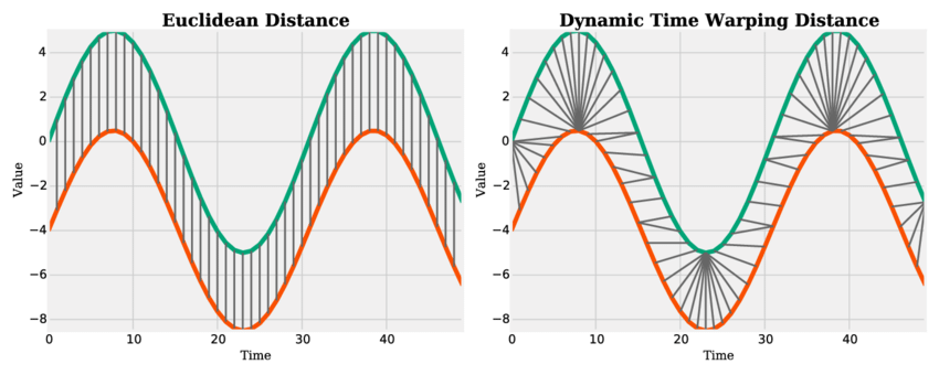Euclidean Distance and Dynamic Time Warping Distance. The latter applies an elastic transformation to the time axis (time warping). Source.

Below is my implementation. I added scaling which I mention later in the post.

def dtw_distance(x, y, d=lambda x,y: abs(x-y), scaled=False, fill=False):
	if fill:
		x = np.nan_to_num(x)
		y = np.nan_to_num(y)
	if scaled:
		x = array_scaler(x)
		y = array_scaler(y)
	n = len(x) + 1
	m = len(y) + 1
	DTW = np.zeros((n, m))
	DTW[:, 0] = float('Inf')
	DTW[0, :] = float('Inf')
	DTW[0, 0] = 0
	
	for i in range(1, n):
		for j in range(1, m):
			cost = d(x[i-1], y[j-1])
			DTW[i, j] = cost + min(DTW[i-1, j], DTW[i, j-1], DTW[i-1, j-1])
			
	return DTW[n-1, m-1]

Afterwards, a new need came up in that project. I needed to cluster time series. I looked up little bit until I realized I can't find an easy implementation for time series clustering such as some practical Python libraries that you can always find for any purpose nowadays. Then I started to make my own. Of course, my naive approach is very straightforward and utilizes DTW. Here is the logic.

Create all cluster combinations. k is for cluster count and n is for number of series. The number of items returned should be n! / k! / (n-k)!. These would be something like potential centers.
For each series, calculate DTW distances to each center in each cluster groups and assign it to the minimum one.
For each cluster groups, calculate total distance within individual clusters.
Choose the minimum.

And, the method of my TrendCluster class for this is below.

def fit(self, series, n=2, scale=True):
    self.scale = scale
    
    combs = combinations(series.keys(), n)
    combs = [[c, -1] for c in combs]

    series_keys = pd.Series(series.keys())
    dtw_matrix = pd.DataFrame(series_keys.apply(lambda x: series_keys.apply(lambda y: dtw_distance(series[x], series[y], scaled=scale))))
    dtw_matrix.columns, dtw_matrix.index = series_keys, series_keys
    for c in combs:
        c[1] = dtw_matrix.loc[c[0], :].min(axis=0).sum()
     
    combs.sort(key=lambda x: x[1])
    self.centers = {c:series[c] for c in combs[0][0]}
    self.clusters = {c:[] for c in self.centers.keys()}

    for k, _ in series.items():
        tmp = [[c, dtw_matrix.loc[k, c]] for c in self.centers.keys()]
        tmp.sort(key=lambda x: x[1])
        cluster = tmp[0][0]
        self.clusters[cluster].append(k)

    return None

Now, it's time for the fun part, how it works...

I chose stock price changes over the time for Apple (AAPL), Twitter (TWTR), Microsoft (MSFT) and Facebook (FB) to demonstrate this and used Open prices for training set and Close prices for test set.

Change of actual stock prices since April 2017

I think it's clear that we would put AAPL and FB in one and MSFT and TWTR in another because of the obvious price differences if we need to create two clusters from these four stocks. Let's see how TrendCluster works.

clusterer = TrendCluster()
clusterer.fit(train.to_dict('list'), n=2, scale=False)
print clusterer.clusters

It prints as...

{'Open_AAPL': ['Open_AAPL', 'Open_FB'], 'Open_MSFT': ['Open_MSFT', 'Open_TWTR']}

However, the main goal is to cluster the trends. The class needs to get distinctive information about the trends regardless of the actual quantity / magnitude / size / price (this varies depending on the variable type). Scaling helps here.

clusterer_scaled = TrendCluster()
clusterer_scaled.fit(train.to_dict('list'), n=2, scale=True) # watch arg 'scale'
print clusterer_scaled.clusters

It prints as...

{'Open_AAPL': ['Open_AAPL', 'Open_MSFT'], 'Open_TWTR': ['Open_TWTR', 'Open_FB']}

The reason of different clustering reveals itself when we look at the scaled prices of aforementioned stocks below. Huge drops can be seen around March and July 2018 on FB and TWTR. Plus, AAPL and MSFT increase less volatilely comparing to others. This explains the different cluster structure here.

Change of scaled stock prices since April 2017

I think it's really cool and just wanted to share with the world.

Epilogue

TrendCluster can also do other things such as assigning new series to clusters. For the entire code and other details, you can refer to my repository.

Please reach me for any questions, comments, suggestions or just to say Hi!

Lastly, share it if you like this Python class;

Trend Clustering

A New Class in Town

Epilogue

Comment